

According to the International Energy Agency, China accounts for 27.9% of global CO2 emissions, with civil aviation carbon emissions accounting for about 1% of this output, making the country the second largest carbon emitter in the global civil aviation transport sector [1]. By the end of 2023, China’s civil aviation transport passenger volume will have reached 620 million, representing an increase of 146.1% from 2012 [1]. The total transport turnover will reach 118.83 billion ton-kilometres, amounting to a year-on-year increase of 98.3% [1]. Although the pollution from the civil aviation industry is relatively smaller than that of other modes of transportation, it continues to grow rapidly, while emission reduction efforts are hindered by high investment requirements, long research and development cycles, and strict safety requirements [1]. According to the International Civil Aviation Organization, airport-related emissions affect the atmospheric environment, and long-term exposure to harmful substances emitted by aircraft threatens human health [2].
Aircraft activities not only exacerbate climate warming and damage the ozone layer by emitting greenhouse gases and pollutants, but also negatively impact the surrounding environment and human health due to noise pollution [2,3]. Studies have shown that exposure to a variety of air pollutants, especially fine particulate matter, increases the risk of cerebrovascular and neuropsychiatric diseases, and aircraft cruise emissions can even lead to premature death [4]. In addition, aircraft produce a large amount of NOx, SO2, CO, hydrocarbons, PM2.5 and PM10, volatile organic compounds, etc. during the landing and take-off (LTO) phase, which significantly affects the environment and health around the airport [5,6].
Although CO is not a greenhouse gas, it can produce pollutants such as ozone through chemical reactions, thereby affecting the climate. Reducing traffic-related PM2.5 and CO in Tianjin was associated with fewer deaths from cardiovascular and respiratory diseases; cumulative deaths from these two causes decreased by 156 and 961, respectively, from 2016 to 2019 compared with 2015 [7]. Long-term low-concentration CO exposure can cause chronic headaches, cognitive impairment, memory loss, etc., while long-term high-concentration exposure can cause permanent heart and nervous system damage [7]. In turn, NO2 has been associated with high mortality and morbidity worldwide, with short-term exposure increasing mortality risk, especially for vulnerable populations [8]. Studies have shown that short-term exposure to PM2.5, NO2, and O3 could be associated with asthma mortality [9]. In addition, NO2 concentration was shown to be closely related to bronchial symptoms and decreased lung function in asthmatic children, with the effect being more pronounced in high temperature environments [10]. Lastly, as one of the main sources of global air pollution, SO2 can aggravate respiratory diseases such as asthma and chronic bronchitis and increase the risk of cardiovascular disease [11,12].
Ats of aircraft emissions, CO, NO2, and SO2, present as potential hazards to air quality, climate change, and human health. Many studies have used emission factor methods to estimate the concentration of pollutants generated by aircraft activities [13–16]. For example, one study combined emission factors and flight trajectories and used atmospheric diffusion models to simulate pollution distribution around airports [13]. Another used chemical transport models to evaluate the impact of emissions from London Heathrow Airport on local air quality [14]. Elsewhere, a multi-pollutant model was used to distinguish the contribution of vehicle and aircraft emissions near airports to NO2 concentrations [15]. One investigation of the emission factors of different LTO stages found that emissions during the take-off stage were significantly higher than those in other stages [16].
Obtaining accurate, up-to-date aviation emission inventories are crucial for analysing the impact of greenhouse gases and air quality around airports. These inventories are usually based on engine certification emission factors, which accurately assess the impact of air quality around airports by considering factors such as fuel flow and engine operating time [17]. Organisations such as NASA and EUROCONTROL have developed the Global Aviation Emissions Inventory and the Aviation Fuel Use and Emissions Inventory System, respectively, to improve the estimation of aviation emissions and provide essential data support for environmental impact and health risk assessments [18,19]. In China, aircraft LTO-stage pollutant emission factors and emission inventories have also been initially established for the Greater Bay Area [20]. The National Earth System Science Data Center has developed the China High Concentration Air Pollutant Dataset to monitor seven near-ground air pollutants, including NO2, SO2 and CO [20,21]. China started late in airport emission research, has limited public data, and has many emission inventories that still rely on historical data, resulting in inaccurate results [22–24].
The integrated exposure-response model (IER) and the global exposure mortality model (GEMM) are commonly used for assessing the long-term health effects of pollutants [25–27]. The IER model was originally used to assess PM2.5 and was later widely used in global disease burden research, while the GEMM model is more adaptable and can handle higher pollution levels and a wider range of population data [28–30]. In one example, a GEMM model was applied to analyse global PM2.5 exposure levels, showing that the GEMM model provides a more accurate health risk assessment in highly polluted areas [28]. However, there are very few quantitative studies on the health effects of NO2, SO2, and CO.
Here, we first adopted a Gaussian diffusion model [31] to calculate the emission concentrations of Chinese airports from January 2006 to December 2023 [32]. Then, we used the average concentration in January 2006 as the threshold and uses the GEMM model to calculate the number of deaths caused by CO, NO2, and SO2 per month from January 2006 to December 2023.W
METHODS
Calculation of CO, SO2, and NO2 concentration
We first gathered monthly aircraft take-off and landing data from January 2006 to December 2023 from the Civil Aviation Administration of China website (Table 1). Using the modified BFFM2-FOA-FPM method (Table 3) and considering the annual proportions of wide-body, narrow-body, and regional aircraft (Table 2), we calculated the average emissions of CO, SO2, and NOX (with NO2 accounting for 5%) for each LTO stage of the aircraft, as well as the total monthly emissions.
Table 1. China’s civil aviation industry monthly take-offs and landings (January 2006 to December 2023)
| Month | ||||||||||||
|---|---|---|---|---|---|---|---|---|---|---|---|---|
| Year | 1 | 2 | 3 | 4 | 5 | 6 | 7 | 8 | 9 | 10 | 11 | 12 |
| 2006 | 118,247 | 110,504 | 119,228 | 120,656 | 126,539 | 122,629 | 136,680 | 142,489 | 137,583 | 137,791 | 127,312 | 127,211 |
| 2007 | 121,821 | 126,292 | 135,154 | 130,628 | 140,190 | 131,458 | 146,051 | 153,390 | 138,215 | 140,864 | 127,610 | 127,025 |
| 2008 | 116,909 | 123,332 | 129,041 | 139,643 | 129,528 | 113,885 | 132,653 | 129,884 | 123,954 | 128,762 | 133,850 | 124,513 |
| 2009 | 128,015 | 133,218 | 126,666 | 137,539 | 135,855 | 137,628 | 141,359 | 169,414 | 152,525 | 160,574 | 147,892 | 149,030 |
| 2010 | 141,046 | 139,605 | 148,263 | 154,396 | 159,285 | 155,408 | 175,752 | 179,242 | 182,538 | 177,581 | 175,591 | 173,860 |
| 2011 | 189,131 | 174,735 | 180,795 | 189,688 | 192,010 | 186,204 | 202,772 | 216,218 | 209,286 | 213,866 | 202,353 | 199,328 |
| 2012 | 195,966 | 186,345 | 207,773 | 207,437 | 203,235 | 204,118 | 229,580 | 234,412 | 225,504 | 223,445 | 219,202 | 217,227 |
| 2013 | 212,311 | 204,328 | 235,294 | 229,034 | 229,496 | 228,613 | 251,008 | 262,983 | 248,277 | 248,319 | 238,235 | 234,454 |
| 2014 | 242,437 | 230,672 | 253,025 | 253,193 | 252,689 | 247,773 | 277,185 | 285,840 | 271,513 | 280,714 | 271,429 | 276,891 |
| 2015 | 272,059 | 271,176 | 298,235 | 288,235 | 290,756 | 281,681 | 310,588 | 325,966 | 303,992 | 317,773 | 304,916 | 307,563 |
| 2016 | 320,168 | 298,319 | 326,471 | 326,471 | 323,109 | 321,008 | 350,420 | 364,706 | 347,479 | 359,664 | 344,118 | 355,462 |
| 2017 | 363,866 | 332,773 | 370,168 | 365,966 | 375,630 | 367,227 | 389,076 | 399,160 | 389,916 | 402,521 | 395,798 | 401,681 |
| 2018 | 394,538 | 376,471 | 425,630 | 421,849 | 419,328 | 413,445 | 435,714 | 449,580 | 426,050 | 443,277 | 424,370 | 433,193 |
| 2019 | 446,218 | 405,462 | 447,899 | 441,597 | 452,941 | 443,697 | 476,050 | 484,454 | 460,084 | 469,748 | 450,420 | 454,202 |
| 2020 | 424,370 | 105,882 | 163,866 | 165,966 | 226,471 | 254,202 | 289,076 | 319,748 | 351,261 | 364,286 | 347,899 | 336,555 |
| 2021 | 266,807 | 210,924 | 374,790 | 386,975 | 385,714 | 328,151 | 361,765 | 206,303 | 289,496 | 307,983 | 219,748 | 257,983 |
| 2022 | 272,269 | 259,244 | 189,496 | 123,950 | 163,445 | 223,950 | 285,714 | 260,504 | 201,261 | 178,992 | 160,924 | 197,059 |
| 2023 | 310,504 | 333,193 | 364,286 | 391,176 | 407,983 | 425,630 | 477,731 | 487,815 | 449,580 | 462,605 | 427,311 | 452,941 |
Table 3. LTO emissions of various gases from different types of aircraft
| Year | Wide-body aircraft ratio | Narrow-body aircraft ratio | Regional aircraft ratio |
|---|---|---|---|
| 2006 | 0.178356713 | 0.70240481 | 0.119238477 |
| 2007 | 0.1280077 | 0.787295476 | 0.084696824 |
Table 2. Percentage of wide-body aircraft, narrow-body aircraft and regional aircraft
| Year | Wide-body aircraft ratio | Narrow-body aircraft ratio | Regional aircraft ratio |
|---|---|---|---|
| 2006 | 0.178356713 | 0.70240481 | 0.119238477 |
| 2007 | 0.1280077 | 0.787295476 | 0.084696824 |
| 2008 | 0.163621922 | 0.727561557 | 0.108816521 |
| 2009 | 0.163621922 | 0.727561557 | 0.108816521 |
| 2010 | 0.141861938 | 0.766941102 | 0.09119696 |
| 2011 | 0.138400454 | 0.766307431 | 0.095292116 |
| 2012 | 0.137063655 | 0.770533881 | 0.092402464 |
| 2013 | 0.134453782 | 0.790849673 | 0.074696545 |
| 2014 | 0.133333333 | 0.802531646 | 0.064135021 |
| 2015 | 0.131698113 | 0.811320755 | 0.056981132 |
| 2016 | 0.13220339 | 0.813220339 | 0.054576271 |
| 2017 | 0.134708738 | 0.811893204 | 0.053398058 |
| 2018 | 0.067326189 | 0.884034075 | 0.048639736 |
| 2019 | 0.145364065 | 0.804347826 | 0.050288109 |
| 2020 | 0.145016654 | 0.803228286 | 0.05175506 |
| 2021 | 0.126052858 | 0.821340747 | 0.052606394 |
| 2022 | 0.126052858 | 0.821340747 | 0.052606394 |
| 2023 | 0.126052858 | 0.821340747 | 0.052606394 |
Next, we calculated the turnover ratio for each airport (average number of take-offs and landings), allowing emissions to be distributed across airports to estimate the LTO emissions for each airport by month. We then averaged the emission flow rate over time by dividing the total emissions by the number of days in the month, hours in a day, and seconds in an hour, resulting in values expressed in g/s. Finally, we employed a Gaussian diffusion model to calculate the monthly average concentrations of CO, SO2, and NO2 at each airport, expressed in μg/m3.
According to the modified BFFM2-FOA-FPM method, the SO2 emitted per unit fuel consumption is fixed, that is, 3.87g of SO2 is emitted per kilogram of aviation kerosene, so this article calculates the sulfur dioxide databased on the turnover and fuel per unit turnover published by the Civil Aviation Administration of China.
According to the emission flow, the average concentration value is calculated by the Gaussian diffusion model, which has been widely applied in calculating emission concentration [31,33]. The Gaussian diffusion model considers the influence of factors such as wind speed and temperature. Its specific steps are as follows:
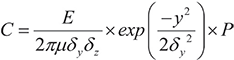

C is the concentration (μg/m3), E is the emission flow (g/s), μ is the wind speed (m/s), this study sets μ = 3.7. δy, δz are the diffusion coefficient of the horizontal and vertical directions, this study sets δy = 1.33, δz = 1. h is the effective height. n is the number of smoke reflections, in this study, h = 2 and n = 3. l is the mixing layer height (m). Generally, for the coastal airports, l = 900, and for the other ones, l = 1100. For the possible emission height that may have effects on humans y, this study selects y = 1, y = 2, and y = 3, and then calculate the average value as the final concentration.
We employed the Gaussian dispersion model because airport-scale air pollution exposure exhibits significant spatial heterogeneity, and existing monitoring stations have extremely limited coverage around airports, making it difficult to directly provide high-resolution continuous concentration fields. Reconstructing the spatial distribution of pollutants using dispersion models is a standard method in health impact assessments of aviation emissions [34]. This type of model has been used in prior studies to simulate near-field pollution from airports and transportation sources [35]. Its basic assumption is that the emission rate is transformed into spatial concentration distribution by parameterising the atmospheric turbulent diffusion process. In the context of airport low-altitude emissions (LTO cycle), it is widely used for near-field exposure assessment of pollutants such as NO2, CO, and SO2, and has been applied in health risk studies at airports in multiple countries. Its rationality has been systematically validated in the literature.
Our analysis focuses not on the precise reconstruction of absolute concentrations, but rather on the relative differences in exposure based on spatial distribution and their attribution for health effects. In this type of health burden study, the role of diffusion models is to provide a high-resolution exposure field, and their uncertainties are typically controlled by subsequent exposure-response functions and uncertainty propagation analysis. We also do not assume that air pollution in airport areas originates solely from aviation activities. In reality, airports and their surrounding environments are influenced by multiple emission sources, including road traffic, auxiliary power units, ground support equipment, nearby industrial activities, and urban background pollution. Accordingly, our aim is not to achieve absolute source attribution, but rather to estimate the incremental contribution of aviation-related emissions using an emissions inventory coupled with a dispersion modelling framework. The concentrations reported here, therefore, do not represent total ambient pollution levels at airports. Instead, they reflect the marginal exposure attributable to aviation activities, derived using standard source apportionment approaches. This methodology is consistent with established practices in the airport health impact assessment literature [31]. To summarise, in complex, multi-source urban environments, precise single-source attribution is rarely achievable based on observational data alone. Consistent with common principles in environmental health research, we adopted a ‘source inventory + dispersion modelling + scenario analysis’ framework to estimate the marginal health impacts of specific emission sources, rather than attempting to fully explain observed pollutant concentrations.
GEMM model
The GEMM functions in two steps: calculating relative risks (RRs) by comparing actual and threshold concentrations and estimating premature deaths using data on population size and baseline mortality rates [36]. This model, which has been widely used in health impact assessments [37–39], predicts hazard ratios for RRs in logarithmic form, extending beyond the observed exposure range, with changes decreasing as exposure increases:

Cg is the actual concentration (μg/m3) and Co is the threshold concentration (μg/m3). Based on existing literature [36], we set C0 = 5. θ, α, μ, and ϑ are the parameters that need to be set in advance. According to the results of parameter sensitivity analysis [26], we set θ at 0.143, α at 1.6, μ at 15.5, and ϑ at 36.8.
Importantly, the GEMM is fundamentally a unified modelling framework built on epidemiological exposure–response functions [26]. Its essence is not limited to PM2.5, but to mapping pollutant exposure levels to health outcomes, typically mortality risk. Although the original GEMM was developed using PM2.5 cohort data, its underlying philosophy is consistent with the IER model, as both rely on a unified nonlinear risk function framework.
In this study, extending the framework to CO, NO2, and SO2 does not involve directly applying PM2.5 parameters, but is supported by two methodological foundations [40,41]. First, independent epidemiological evidence provides pollutant-specific exposure–response relationships. Projects such as World Health Organization (WHO) HRAPIE and multinational cohort studies offer concentration–response functions or relative risk estimates for these pollutants, forming a basis for constructing tailored exposure–response functions. Second, a continuous risk function consistent with GEMM is adopted, rather than threshold or linear cutoff models, ensuring comparability and additivity of health effects across pollutants within a unified framework. This enables a coherent assessment of multi-pollutant health burdens and aligns with established practices in the literature.
Concentration threshold settings for air pollutants vary substantially across countries and regions. For NO2, the World Health Organization recommends that the one-hour average concentration should not exceed 200 μg/m3 to protect public health [42]. Similarly, the European Union sets a one-hour threshold of 200 μg/m3, while additionally specifying an annual average limit of 40 μg/m3 [43].
For carbon monoxide (CO), the WHO recommends an eight-hour average concentration limit of 9 mg/m3 and a one-hour limit of 10 mg/m3 [42]. Consistently, the US Environmental Protection Agency establishes a national standard with an eight-hour average threshold of 9 mg/m3 [44]. For sulfur dioxide (SO2), WHO guidelines suggest that the 24-hour average concentration should not exceed 20 μg/m3, and the one-hour average should remain below 500 μg/m3 [42]. In contrast, the EU defines a one-hour threshold of 350 μg/m3 and a 24-hour threshold of 125 μg/m3 [45]. These discrepancies highlight the lack of global uniformity in air quality standards and complicate cross-regional comparisons.
To address this inconsistency, we adopted January 2006 as a unified reference point and evaluated mortality changes relative to that baseline. Rather than relying on externally defined thresholds, this approach standardises the analytical framework for CO, NO2, and SO2, thereby enhancing the comparability of results. Following a screening process, we selected 126 airports as representative of national-level aviation systems. We used the average pollutant concentrations observed in January 2006 as baseline levels, and applied the GEMM framework to estimate monthly mortality from January 2006 to December 2023, disaggregated by gender and age.
In environmental epidemiology, three main approaches are typically used to define counterfactual exposure baselines: the theoretical minimum risk exposure level; low-end distributional benchmarks (e.g. the 5th percentile); and the average conditions during a stable historical period. We adopted the third approach in our analysis, as the use of theoretical minimum risk exposure level or low-percentile thresholds would have introduced inconsistencies across pollutants and regions due to the substantial spatial imbalance in long-term observational data for CO, NO2, and SO2 across global airports. In contrast, selecting a common historical reference point enables the construction of a structurally consistent baseline across all airports and pollutants, thereby preserving the additivity and spatial comparability of multi-pollutant health impacts.
We selected January 2006 as the baseline based on three considerations. First, it represents a relatively stable phase in global aviation activity, prior to subsequent rapid growth and major policy interventions, and can therefore be viewed as a ‘low-disturbance’ reference state [46]. Second, data coverage for all airports and pollutants was complete during this period, minimising bias from missing observations. Third, we did not interpret the baseline concentration as a health-based safety threshold.
Health effect estimation remains strictly grounded in the continuous exposure–response relationships defined within the GEMM framework. Accordingly, deviations from the baseline, whether increases or decreases, are interpreted as changes in excess risk associated with relative exposure increments, rather than absolute risk thresholds.
We used the following equation for the number of premature deaths:
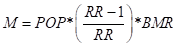
Here, RR is the relative risk, POP is the population, BMR is the base mortality rate, and M is the number of premature deaths.
We obtained the base mortality rate of various diseases from the Global Burden of Disease (GBD) dataset [47], and the population data within 50 km of the airport from the LandScan dataset [48]. Given the lack of high-resolution mortality data at the airport scale, we adopted a simplifying assumption that disease-specific mortality rates are spatially uniform at the national level during the study period. Under this assumption, we used age- and sex-specific national mortality estimates from the GBD as baseline values, which we then spatially allocated according to population distribution. Otherwise, we retained population size data and its share of the national total within the study area (defined as a 50 km radius around each airport) from the LandScan dataset. We subsequently applied these population proportions to the national-level, age- and sex-specific mortality totals from the GBD to estimate baseline mortality for populations residing near airports. This approach implicitly assumes that baseline mortality risk per capita does not vary systematically across regions. In terms of temporal resolution, as GBD mortality data are primarily reported on an annual basis, so we assumed that baseline mortality is evenly distributed throughout the year. Annual mortality rates are therefore converted into temporally uniform estimates to align with pollution exposure data at monthly or finer time scales.
The effects of factors such as wind speed, humidity and temperature on concentration have already been considered in the concentration calculation process [31], so we did not repeatedly consider them when calculating health effects. Furthermore, we defined a 50 km population buffer centred on each airport to represent the population potentially affected by aviation-related emissions. This spatial scale is selected based on two considerations. First, a prior study has indicated that emissions associated with airport operations – particularly during take-off and landing, as well as the formation of secondary pollutants – can influence air quality over distances of several tens of kilometres [49]. Second, a 50 km buffer ensures adequate population coverage while avoiding statistical instability that may arise from overly small spatial units. As such, this choice reflects a balance between spatial representativeness and statistical robustness.
To address spatial overlap between adjacent airport buffer zones, we applied a population deduplication (or distance-/weight-based allocation) procedure to avoid double counting. Specifically, when a population grid cell falls within multiple buffer zones, it is either counted only once or allocated based on proximity (e.g. nearest-airport assignment). This ensures national-level population consistency and prevents systematic overestimation of attributable mortality.
RESULTS
Temporal trends in CO concentrations and CO-attributable mortality
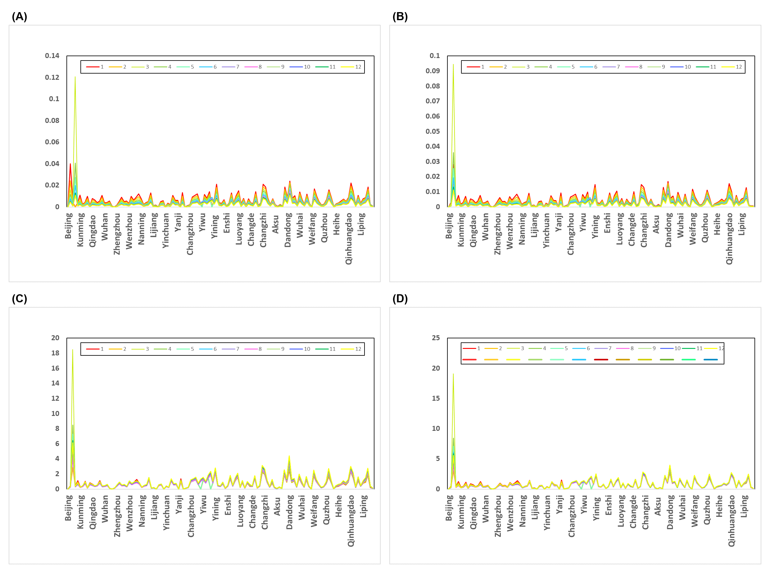
From 2006 to 2019, CO concentrations at Chinese airports increased continuously. Concentrations then declined substantially during 2020-2022 and reached a minimum of 34,857.46 μg/m3 in 2022. In 2023, CO concentrations rebounded by 33,072.62 μg/m3 relative to 2022, representing a 94.9% increase. CO-attributable mortality was highest among men aged 75–79 and women aged 80–84 years. The largest numbers of deaths were observed in winter and early spring, with peaks in February and March 2006 and the fewest deaths in October and December. In 2023, monthly deaths peaked in November and December among men and in January among women (Figure 1).
Figure 1. Deaths from cardiovascular disease due to changes in CO concentration. Increase in cardiovascular deaths in men (Panel A) and women (Panel B) younger than 5 years of age per unit increase in CO concentration at each airport in 2023. Number of cardiovascular deaths in men (Panel C) and women (Panel D) aged 80-84 years due to CO at each airport in 2023.
Temporal trends in NO2 concentrations and NO2-attributable mortality
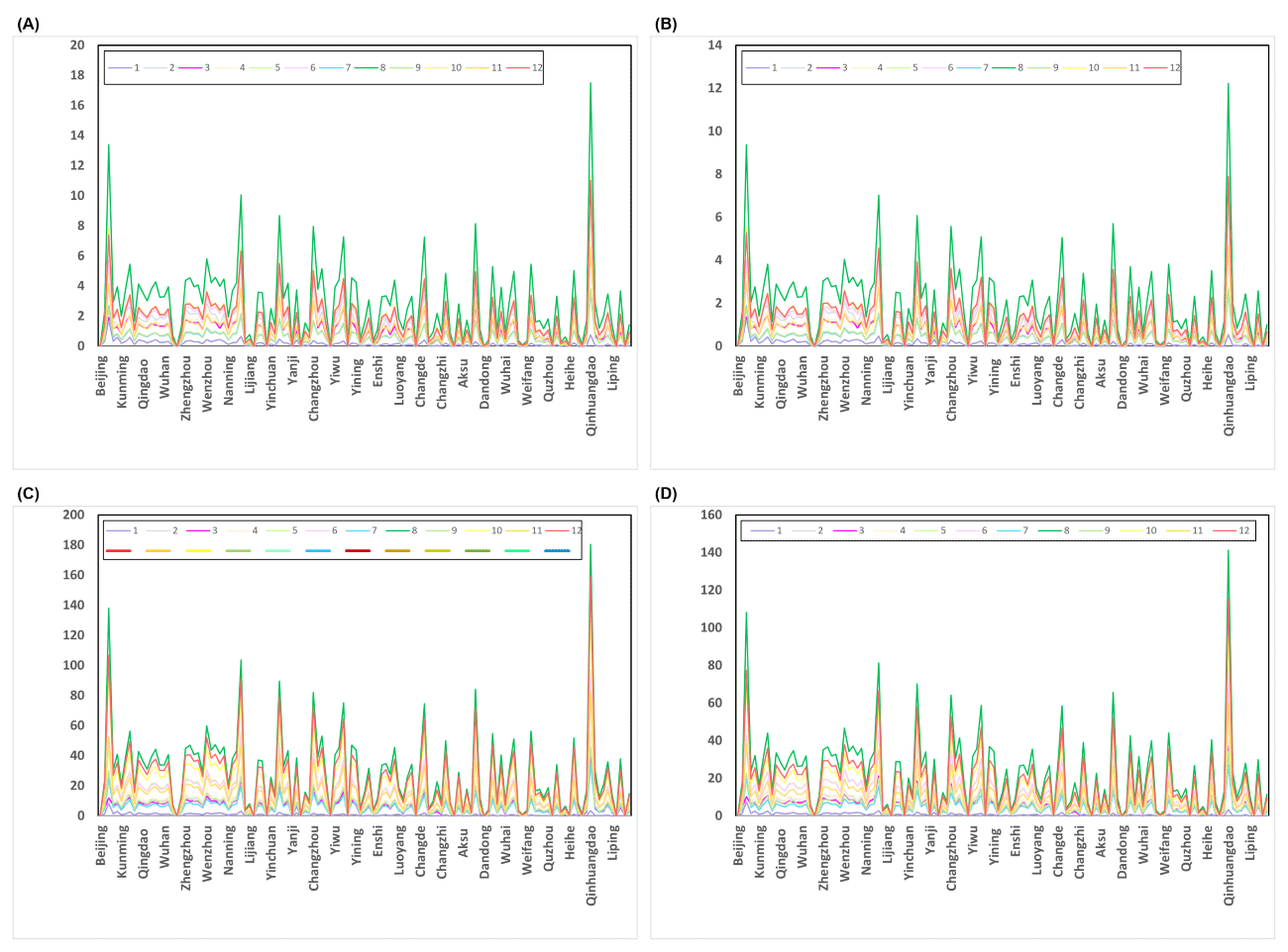
From 2006 to 2023, NO2 concentrations at airports followed a pattern similar to that of CO and reached their highest annual level in 2019. Between 2019 and 2022, NO2 concentrations decreased from 4744.27 μg/m3 to 1902.99 ug/m3 and then increased to 3708.54 μg/m3 in 2023. The highest numbers of respiratory disease deaths attributable to NO2 were observed in summer, with a peak in August (Figure 2).
Figure 2. Deaths from respiratory diseases due to changes in NO2 concentrations. Increase in respiratory disease deaths per unit increase in NO2 concentration at airports in 2023, in men (Panel A) and women (Panel B) younger than 5 years, and men (Panel C) and women (Panel D) aged 80-84 years.
Temporal trends in SO2 concentrations and SO2-attributable mortality
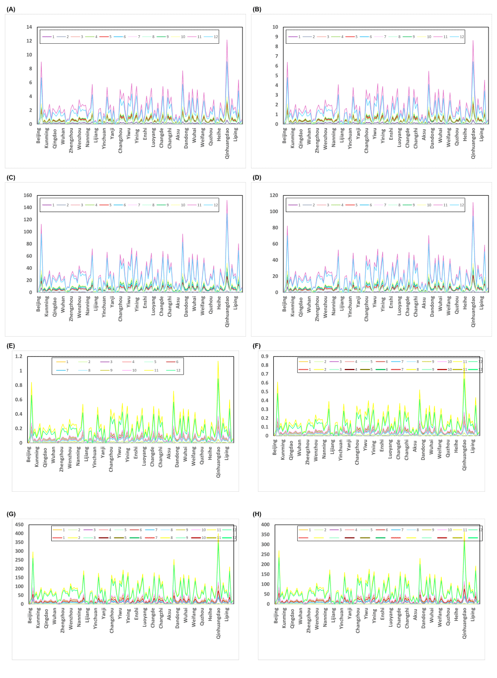
SO2 concentrations at airports also peaked in 2019 at 16,010.34 μg/m3 and then decreased to 6949.63 μg/m3 in 2022, close to the 2009 level. In 2023, the estimated change in deaths was negative in some months relative to the January 2006 baseline. SO2-attributable respiratory deaths were highest in November, December, and June, and the mortality burden was greatest in older age groups, particularly men. For deaths associated with unit increases in SO2 concentration in 2006 and 2023, the largest increases were observed in November and December. Among adults aged 80–84, the number of attributable deaths was particularly high, and among those aged >85 years, women had higher mortality than men (Figure 3).
Figure 3. Deaths from respiratory diseases and cardiovascular diseases due to changes in SO2 concentrations. Increase in respiratory disease deaths per unit increase in SO2 concentration at each airport in 2023, in men (Panel A) and women (Panel B) younger than 5 years, and men (Panel C) and women (Panel D) aged 80-84 years. Increase in cardiovascular disease deaths per unit increase in SO2 concentration at airports in 2023, in men (Panel E) and women (Panel F) younger than 5 years, and men (Panel G) and women (Panel H) aged 80-84 years.
Airport-level distribution of pollutant burden in 2023
Across airports, Guangzhou Baiyun, Shanghai Pudong, Beijing Capital, Shenzhen Baoan, and Chengdu Tianfu ranked as the top five for CO, NO2, and SO2 burden in China (Figure S1 in the Online Supplementary Document). In 2023, Guangzhou Baiyun recorded the highest pollutant concentrations, with CO, NO2, and SO2 concentrations of 3231.19 μg/m3, 176.40 μg/m3, and 667.48 μg/m3, respectively. At Shanghai Pudong, the corresponding concentrations were 2476.81 μg/m3, 135.22 μg/m3, and 511.64 μg/m3, and at Beijing Capital they were 1910.28 μg/m3, 104.29 μg/m3, and 394.61 μg/m3. In 2023, Shanghai Pudong recorded six CO-attributable cardiovascular deaths, compared with two at Guangzhou Baiyun.
Age- and sex-specific patterns of attributable mortality
From 2006 to 2023, CO-attributable cardiovascular deaths were highest among women aged 80-84 and men aged 75–79, whereas the lowest burden was observed among children aged 5–9. Cardiovascular deaths attributable to CO were higher in women aged >85 years than in men of the same age group (Figure S2, Panels A and B in the Online Supplementary Document). The number of attributable deaths declined after age 80 years in men and after age 85 years in women. The largest annual increase in CO-attributable cardiovascular deaths occurred in 2019, with 156,518 additional deaths in men and 115,610 in women.
From 2006 to 2023, NO2-attributable respiratory deaths varied across age groups and were highest in 2019, particularly among individuals aged 80–84. Men were generally more affected than women, although in 2023 women aged >90 years showed a greater increase in mortality than men (Figure S2, Panel B in the Online Supplementary Document). Attributable mortality was relatively low among individuals aged ≥90 years, whereas the attributable burden was higher among children aged <5 years.
SO2-attributable deaths were observed for both respiratory and cardiovascular diseases, with a larger number of attributable deaths recorded for cardiovascular disease. The attributable mortality burden was highest in older age groups, with peaks among men aged 75–79 and women aged 80–84. In contrast, respiratory deaths attributable to SO2 were more concentrated among children aged <5 years. The highest numbers of attributable deaths were observed in 2019, followed by 2018. At very old ages, females showed a higher attributable mortality burden than males for respiratory disease (e.g. ≥90 years) and cardiovascular disease (e.g. ≥95 years) (Figure S2, Panels E–L in the Online Supplementary Document).
DISCUSSION
Our analysis covered 126 airports which were intended to represent national-level airport activity. Based on estimated emissions of CO, SO2, and NO2 from 2006 to 2023, we conducted a modelling-based assessment to evaluate the potential health impacts associated with aviation-related air pollution. Our results are thus derived from an integrated framework combining emission inventories, dispersion modelling, and transferred exposure–response functions, and therefore represent estimated health risks under specific modelling assumptions, rather than directly observed or causal mortality outcomes [34,49–51].
The temporal analysis suggests that modelled concentrations of all three pollutants peaked around 2019, with an overall increase from 2016 to 2019 after an earlier decline. The year 2019 also corresponded to the largest modelled increases in mortality across pollutants. This pattern is plausible because airport operations can measurably elevate near-surface pollutant concentrations in surrounding communities, while aviation-related impacts may extend beyond the immediate runway environment [51,52].
The estimated health impacts were generally higher in males than in females across most scenarios. Within the model results, CO was associated with relatively larger estimated impacts on respiratory mortality than SO2 and NO2, while NO2 showed smaller effects in this category. By age, the modelled impacts of CO on cardiovascular mortality were concentrated among older populations, with the highest estimates observed among females aged 80–84 and males aged 75–79, and the lowest impacts among children aged 5–9 years. For SO2 and NO2, the modelled respiratory impacts were also concentrated in vulnerable age groups, with NO2 showing relatively larger estimated effects among those aged 80–84 and children under 5 years of age. For SO2-related cardiovascular mortality, the highest impacts were observed among males aged 75–79 and females aged 80–84, while younger populations were less affected. Such sex-related heterogeneity is consistent with prior calls to incorporate sex and gender as effect modifiers in air-pollution epidemiology, although the direction and magnitude of the differences vary across studies [53–55].
Seasonal variation was also evident, with stronger CO-related mortality increments in winter and early spring. From a temporal perspective, the largest modelled increases in respiratory mortality for NO2 occurred in August, the strongest CO-related increases in cardiovascular and cerebrovascular mortality occurred from November to January, while SO2 showed the largest cardiovascular effects in November and December. Seasonal effect modification has been reported previously in time-series studies of outdoor air pollution and mortality, likely reflecting season-dependent meteorology and exposure patterns [54]. These results are broadly compatible with the wider literature showing positive associations between NO2, SO2, and CO exposure and mortality outcomes. For CO specifically, a nationwide time-series analysis in 272 Chinese cities reported increased cardiovascular mortality per 1 mg/m3 increase and no clear threshold [56]. while recent systematic reviews and meta-analyses support pollutant-specific concentration-response functions for NO2 and SO2 [57,58].
Our provides a nationwide, airport-centred assessment of the health burden associated with aircraft-related emissions of CO, SO2, and NO2 by integrating modelled pollutant concentrations, population distribution, and concentration-response relationships, thereby offering a consistent basis for comparing relative health burdens across regions and population groups [34,50]. Rather than establishing new causal relationships, the analysis applies an existing exposure–response framework to quantify relative health burden around airports. The baseline concentration is best understood as a reference condition rather than a health-based safety threshold. More broadly, burden of disease studies typically rely on established concentration-response functions and integrated risk models, such as IER and GEMM, because they provide a coherent way to translate exposure into health risk across concentration ranges [26,27,40].
Several limitations should be acknowledged. The analysis depends on modelled concentrations and downscaled mortality rates, so uncertainties in emission inventories, dispersion parameters, population allocation, and spatial resolution remain. Source attribution is also imperfect in densely populated regions with multiple overlapping emissions. In addition, the generalised concentration-response functions introduce uncertainty, particularly for gaseous pollutants, which remain less extensively characterised than PM2.5, although the current evidence base does support quantitative burden estimation [56–58]. Future work should incorporate higher-resolution exposure estimates, sensitivity analyses of key model parameters, and observational health data where available.